In this article, we present a Scala implementation of a purely functional random access list; a functional data structure which was first presented by Chris Okasaki in this paper.

The random access list data structure supports array lookup and update operations in O(log n) time, and simultaneously provide O(1) time cons, tail and head list operations.

Lists are central to functional programming. They are convenient and well suited to implement recursive algorithms. However, for applications which need random access to data, they become inefficient, because accessing the iᵗʰ element in a list, requires O(i) time. Arrays, on the other hand, are very fast when it comes to randomly looking-up elements, but they can prove very awkward in a functional programming setting. Arrays are mutable data structures which destruct their data once updated. Also, their efficiency is tied to the assumption that they are used in a single-threaded environment. To that end, random access lists are the best of both worlds. They are immutable data structures that can be used safely in multithreaded environments without sacrificing the random access efficiency. Next, we’ll see how that can be achieved.

Complete Binary Trees

A complete binary tree is a binary tree which has a root node and two totally balanced subtrees, the left subtree and the right subtree. Thus, the number of nodes in a complete binary tree is a skew binary number of the form 2ᵏ -1, where k is a positive integer (see figure 1).

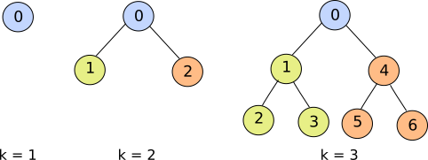
Figure 1. Complete binary trees for k = 1, 2, and 3.

As the complete binary tree will be our basic building block in implementing the random access list, we’ll start by implementing the complete binary tree as an algebraic data type.

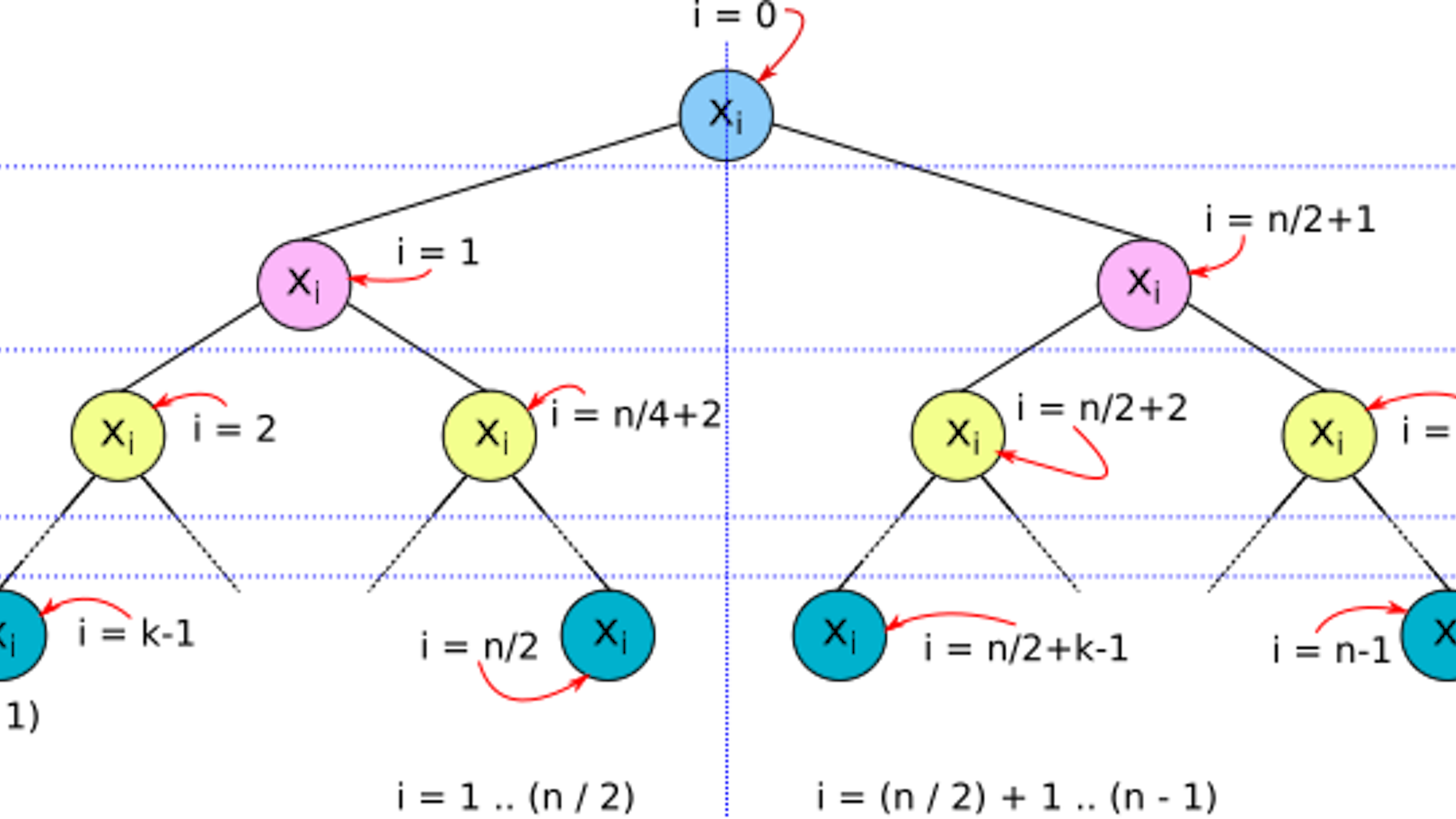
First we must understand how values are stored in a complete binary tree. For a list of values of size n, (x₀, x₁, …, xn-₁), where n is a skew binary positive integer, x₀ is stored at the tree root, x₁… xn/₂ are stored at the left subtree, and x(n/₂)+₁… xn-₁ are stored at the right subtree (see figure 2).

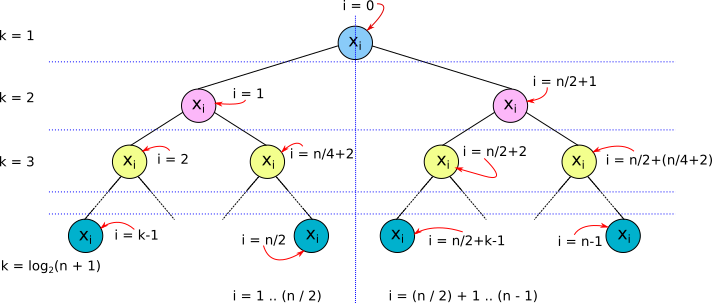
Figure 2. Storing values in a complete binary tree.

Other arrangements are possible, but this particular arrangement will prove advantageous in our implementations of basic array and list operations.

A complete binary tree may be represented in code as¹:

sealed trait CompleteBinaryTree[A] {
  def lookup(size: Int, index: Int): A = (this, index) match {
    case (Leaf(x), 0)                        => x
    case (Leaf(_), _)                        => throw new Exception("Index is not in list.")
    case (Node(x, _, _), 0)                  => x
    case (Node(x, l, _), i) if i <= size / 2 => l.lookup(size / 2, i - 1)
    case (Node(x, _, r), i) if i > size / 2  => r.lookup(size / 2, i - 1 - size / 2)
  }
  def update(size: Int, index: Int, y: A): CompleteBinaryTree[A] = (this, index) match {
    case (Leaf(_), 0)                        => Leaf(y)
    case (Leaf(_), _)                        => throw new Exception("Index is not in list.")
    case (Node(_, l, r), 0)                  => Node(y, l, r)
    case (Node(x, l, r), i) if i <= size / 2 => Node(x, l.update(size / 2, i - 1, y), r)
    case (Node(x, l, r), i) if i > size / 2  => Node(x, l, r.update(size / 2, i - 1 - size / 2, y))
  }  
}

object CompleteBinaryTree {
  def apply[A](xs: List[A]): CompleteBinaryTree[A] = {
    def inner(xs: List[A], size: Int): CompleteBinaryTree[A] = size match {
      case 1 => Leaf(xs.head)
      case s if Math.pow(2, Math.floor(Math.log(s + 1)/ Math.log(2))).toInt == s + 1 => {
        val t = xs.tail
        val s_ = size / 2
        Node(xs.head, inner(t.take(s_), s_), inner(t.drop(s_), s_))
      }
      case _ => throw new Exception("Size is not a skew binary.")
    }
    inner(xs, xs.length)
  }
}
case class Leaf[A](value: A) extends CompleteBinaryTree[A]
case class Node[A](value: A, l: CompleteBinaryTree[A], r: CompleteBinaryTree[A]) extends CompleteBinaryTree[A]

Listing 1. Scala implementation of complete binary trees.

The CompleteBinaryTree polymorphic type is represented as a sealed trait(listing 1). Thus, all data constructors of CompleteBinaryTree are required to be declared here; namely Node and Leaf. A tree of type Leaf is a singleton tree. A tree of type Node contains two subtrees: a lift subtree and a right subtree. Since, in this article, we are only concerned about complete binary trees, which are totally balanced, the two subtrees of a Node must be either Nodes or Leafs.

Now, we consider the implementations of the two basic array operations: lookup() and update(). The lookup() function uses pattern matching to produce the output value depending on the type of the CompleteBinaryTree and the index of the value being searched for. If the CompleteBinaryTree is a Leaf, the value contained in the Leaf is returned as it is the only value there is. However, if the index supplied to lookup() is not 0, an exception is thrown, because a Leaf is a singleton tree. If the CompleteBinaryTree is a Node, the value at the root of the tree is returned if the index supplied to lookup() is 0. If index is not 0, and index ≤ size / 2 , where size is the size of the tree, then the required value must be in the left subtree (see figure 2). In this case lookup() calls itself recursively supplying the left subtree as the tree together with updated values for index and size. Finally, if index > size / 2, lookup() , again, calls itself, recursively. Only this time, the supplied values to the call is the right subtree and updated values for index and size.

The update() function works in similar way to the lookup() function, but it returns a new CompleteBinaryTree updated at the index supplied in the call with the new value specified in same call. If the tree being updated is a Leaf, a new Leaf is returned with its only value updated to match the new value supplied by the caller. However, that is only possible, if index is 0, otherwise an exception is thrown as before. If the tree is a Node, index is checked to determine which subtree is going to be updated. The update() function returns a new Node, which consists of the root of the old Node, one of the two old subtrees depending on the values of index and size, and an updated subtree generated by a recursive call to update(). Note that update() always return a new data structure and doesn’t mutate the old data structure. This immutable approach to updating data structures is an essential pillar of pure functional algorithm design.

It is worth noting that because the height of a complete binary tree is logarithmic in its size (see figure 2), the two array operations run in O(log n) time.

The companion object to CompleteBinaryTree declares a convenient function, apply(), which is useful in constructing a CompleteBinaryTree from an ordinary List. Function apply() checks the size of the input list, to determine if the list has one or more elements. If there is only one element in the list, a Leaf is generated to wrap the only value in the list. If there are more than one element in the list, the head of the list is used to populate the root of a Node . The tail of the list is, then, divided into two equal lists which are used to construct the left and right subtrees of the Node through two recursive calls to inner(). Note that function inner() is used by apply() to do the heavy lifting. The convenient Scala syntax CompleteBinaryTree(List(....)) is used when calling apply(), which will throw an exception if the length of the supplied list is not a skew binary number. The length of the list is calculated once by apply() and then supplied to inner() to avoid the cost of calculating the list length several times.

It might be tempting to think that a CompleteBinaryTree is enough to construct our target data structure, the random access list, but the limitation on the size of the input list is a serious one. We need to have a way to start with an ordinary list of arbitrary size and end up with a random access list. We’ll see how, next.

A Full-Fledged Random Access List

To represent lists of arbitrary sizes, one can utilize a list of complete binary trees instead of just one tree. We know this is possible, because an empty list can be represented by an empty list of complete binary trees and any other list of arbitrary size > 0 can be represented by size number of singleton trees. However, we are going to use one specific decomposition of size called the greedy skew-binary decomposition (GSBD).

A skew-binary decomposition of a natural number is said to be greedy if the largest term in the decomposition is as large as possible and the rest of the decomposition is also greedy. For example, the GSBD of 28 is [3, 3, 7, 15], as shown in figure 3.

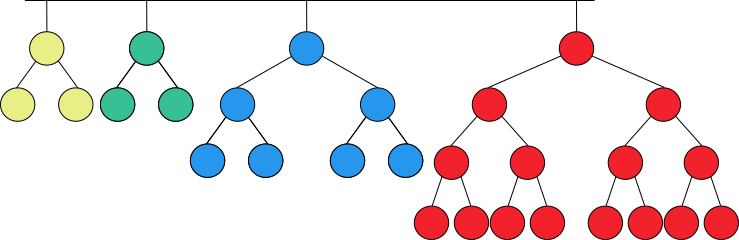
Figure 3. Greedy skew-binary decomposition of 28.

The above recursive definition of GSBD can be used to devise an algorithm to generate g(n), the GSBD of the natural number n. The algorithm is straightforward as shown by the below Scala code:

package greedySkewBinary
object Gen {
  def g(n: Int): List[Int] = {
    def loop(n: Int, acc: List[Int]): List[Int] = {
      import Math._
      if (n == 0) acc else {
        val term = pow(2, floor(log(n + 1) / log(2))).toInt - 1
        loop(n - term, term::acc)
      }
    }
    loop(n, List())
  }
}

Function g() accepts an Int, n, for which it outputs the GSBD as a List[Int]. Internally, g() uses a function loop() to do the actual work. Function loop() uses an accumulator, acc, to memorize the decomposition terms between its successive calls to itself. When n == 0, acc is returned, otherwise, loop() calculates the next term of the decomposition and calls itself supplying n  - term as the new Int to be decomposed, together with an acc that has been updated with the newly calculated term. All g() has to do, is to call loop() supplying n as the Int to be decomposed an and empty List as the initial value of the accumulator.

Despite the simplicity of the above algorithm, it can be used to deduce some important properties of GSBDs, in general:

1. The algorithm is deterministic. In other words, it will always produce a decomposition no matter the value of n as long as n ≥ 0. Thus, every natural number has a greedy skew-binary decomposition.
2. Let us assume that there exist two different GSBDs of a natural number n, g₁(n) and g₂(n). By definition, the largest term in g₁(n), T₁, and the largest term in g₂(n), T₂, must be the same. The remaining of the two decompositions, g₁(n-T₁) and g₂(n-T₂), are also greedy, by definition. Hence, the second largest term in g₁(n) and the second largest term in g₂(n) must be also the same, and so on. We conclude that g₁(n) and g₂(n) must be the same. Thus, every natural number has a unique greedy skew-binary decomposition.
3. Let us assume that two successive terms tᵢ, and tᵢ+₁ of the GSBD of n, g(n), are equal. In the algorithm that we used before to generate g(n), this means that tᵢ+₂ is calculated by supplying (tᵢ+₁)-tᵢ to the next iteration of the algorithm as the number to be decomposed. But, (tᵢ+₁)-tᵢ = 0; hence, the algorithm terminates. Thus, all terms of a greedy skew-binary decomposition are unique except for the two smallest terms (the first two terms in the ascending ordering of the decomposition terms), which may be equal.
4. We have shown before that we can do lookup and update operations on a complete binary tree in O(log n) time. But how about if we want to lookup or update a value in a list of complete binary trees? Well, it turns out that if the list terms are the GSBD of the list's size, we are still able to do lookup and update operations in O(log n) time. To show that this is possible, we must find the upper limit on the number of terms in the GSBD of n, g(n). We know that g(n) terms are all skew-binary numbers ≤ n. We also know from property 3 above, that they must be all unique except for the smallest two of them which may be repeated. Assuming that g(n) contains all the skew-binary numbers which are > 0 and ≤ n with the smallest term repeated, g(n) will have k+1 terms where 2ᵏ-1 is the largest skew binary number ≤ n. Because we know that k is an integer, k + 1=⌊log₂(n+1)⌋ + 1. Note that for log₂(n+1) to be an integer, n must be a skew-binary number, in which case g(n) will consist of only one term, namely, 2ᵏ-1. Obviously, this case is not useful in our search for the upper limit on the number of terms in g(n). We can safely assume that log₂(n+1) is not an integer. Thus, the upper limit, we are looking for is k + 1=⌊log₂(n+1)⌋ + 1 = ⌈log₂(n+1)⌉. Thus, the maximum number of trees in the list, k+1, is logarithmic in the total number of elements n, which means that locating the right tree for lookup and update operations can be done in O(log n) time.
5. Finally, we consider the relation between g(n) and g(n+1). This is important because it gives us a way to implement two important list operations, cons() and tail(). Let g(n) = [t₀, t₁, …, T₁, T₀] and g(n + 1) = [t₀', t₁',…, T₁', T₀']. If T₀≠T₀', then n+1 must be a skew-binary number and hence g(n) = [n/2, n/2] and g(n+1) = [n + 1]. If T₀=T₀', then g(n-T₀) = [t₀, t₁, …, T₁] and g(n+1-T₀)=[t₀', t₁',…, T₁']. If T₁≠T₁', then n+1-T₀ must be a skew-binary number and hence, g(n-T₀)=[(n-T₀)/2, (n-T₀)/2] and g(n+1-T₀)=[(n-T₀)+1], and so on. We conclude that, if t₀ = t₁, then g(n+1) = [[1,t₀, t₁], t₂, ..]; and if t₀ ≠ t₁, then g(n+1)=[1,t₀, t₁,…].

We can take advantage of property 5 to implement efficient cons() and tail() operation. In cons(), we are adding an element to the front of the list. If the GSBD of the original list’s size is g(n) then the GSBD of the resulting list’s size is g(n+1). The opposite is true in the case of tail(). If the GSBD of the list’s size is g(n+1), then the GSBD of it tail’s size is g(n) (see figure 4).

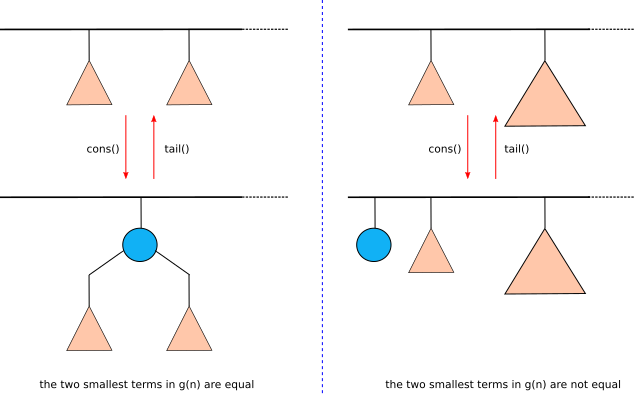
Figure 4. How cons() and tail() operations work on a random access list.

Now, it is time to show the code for the RandomAccessList (listing 2).

object RandomAccessList {
  type RandomAccessList[A] = List[(CompleteBinaryTree[A], Int)]

  def fromList[A](xs: List[A]): RandomAccessList[A] = {
    def sublists[A](xs: List[A]): List[(List[A], Int)] = {
      def inner(xs: List[A], size: Int, acc: List[(List[A], Int)]): List[(List[A], Int)] = size match {
        case 0 => acc
        case s => {
          val s_ = Math.pow(2, Math.floor(Math.log(s + 1) / Math.log(2))).toInt - 1
          inner(xs.take(s - s_), s - s_, (xs.drop(s - s_), s_)::acc)
        }
      }
      inner(xs, xs.length, List())
    }
    sublists(xs) map {pair => (CompleteBinaryTree(pair._1), pair._2)}
  }

  def lookup[A](ral: RandomAccessList[A], index: Int): A = ral match {
    case Nil                                => throw new Exception("Index is not in list.")
    case (tree, size)::_ if index < size    => tree.lookup(size, index)
    case (_, size)::tail if index >= size   => lookup(tail, index - size)
  }

  def update[A](ral: RandomAccessList[A], index: Int, y: A): RandomAccessList[A] = ral match {
    case Nil                                 => throw new Exception("Index is not in list.")
    case (tree, size)::tail if index < size  => (tree.update(size, index, y), size)::tail
    case (tree, size)::tail if index >= size => (tree, size)::update(tail, index - size, y)
  }

  def cons[A](ral: RandomAccessList[A], e: A): RandomAccessList[A] = ral match {
    case (tree1, size1)::(tree2, size2)::tail if size1 == size2 => (Node(e, tree1, tree2), size1 + size2 + 1)::tail
    case (tree1, size1)::(tree2, size2)::tail if size1 != size2 => (Leaf(e), 1)::(tree1, size1)::(tree2, size2)::tail
    case ts                                                     => (Leaf(e), 1)::ts
  }

  def head[A](ral: RandomAccessList[A]): A = ral match {
    case Nil                      => throw new Exception("Head of empty list.")
    case (Leaf(x), _)::tail       => x
    case (Node(x, _, _), _)::tail => x
  }

  def tail[A](ral: RandomAccessList[A]): RandomAccessList[A] = ral match {
    case Nil                         => throw new Exception("Tail of empty list.")
    case (Leaf(_), _)::tail          => tail
    case (Node(_, l, r), size)::tail => (l, size / 2)::(r, size / 2)::tail
  }
}

Listing 2. Scala Implementation of Random Access List.

As seen in listing 2, RandomAccessList is just a type alias for List[(CompleteBinaryTree, Int)]. The Int type parameter is the size of the CompleteBinaryTree. Function fromList() transforms an ordinary List into a List of Lists. Each sublist is a CompleteBinaryTree of size equal to the corresponding term in the GSBD of the input List’s size. The previously mentioned algorithm which generates GSBDs, is used by toList() to generate the CompleteBinaryTrees (the sublists of the output List).

Function lookup() uses the supplied index to check if the element being searched for is in the first subtree. If so, it calls CompleteBinaryTree’s lookup() function to return the element. If not, it calls itself supplying the tail of the input List together with an updated value of index. Function update() works in a similar way to lookup(), but it calls CompleteBinaryTree’s update() function, instead of its lookup(). Both lookup() and update() run in O(log n) time. O(log n) to locate the right subtree and O(log n) to locate the right element within the subtree.

If the first two elements of the input List are equal, cons() turns them into the left and right trees of a newly created Node, respectively. At the root of the Node, cons() stores the element supplied by the caller, e.The newly created Node is the first element in the resulting RandomAccessList. If the input List has more elements beyond the second element, they will represent the tail of the RandomAccessList; otherwise the tail will be an empty List (Nil). If the first two elements of the input List are not equal, or if the input List’s size is < 2, the whole input list will represent the tail of the resulting RandomAccessList, while its head will be a Leaf containing e. Note that cons() requires O(1) running time.

Function head() also requires O(1) running time and will always return the value contained by the first element in the input List (except when the input List is Nil, in which case an exception is thrown).

Function tail() checks if the head of the input List is a Leaf. If so, it just returns the the input List’s tail. Otherwise, if the head of the input List is a Node, a RandomAccessList is returned with the left and right trees of Node representing the first and the second element of the resulting RandomAccessList, respectively; and the tail of the input List representing the remaining elements of the RandomAccessList. Clearly, tail() requires O(1) running time.

We conclude that list operations on a RandomAccessList require O(1) time while array operations require O(log n) time. It gets even better when we note that locating the iᵗʰ element in a CompleteBinaryTree requires O(log i) time. Also, if we assume that a RandomAccessList contains one CompleteBinaryTree of every size < n, then the iᵗʰ element of the list will be in the log(i)ᵗʰ tree, approximately. Which means that locating the right tree requires O(log i) time, too. In fact, this approximation remains good even if we have some missing trees but not if we have large gaps. While it can be shown that the probability of having large gaps is very low for randomly chosen n, we feel it is intuitive. Thus, array operations on RandomAccessList require O(log i) time in the expected case and O(log n) time in the worst case.

¹ The code in this article is available on github